#PCA is your friend, part two

Continued from the post below

The loadings the thing, wherin I’ll catch the essence of the dataset. Principal component analysis (PCA) is an excellent, and often essential, method for analysing a large amount of data. Our research question centers around the differences between two fossil sites, and the large dataset we have at hand is made up of x-ray fluorescence spectra from fossil bones. These data go into the PCA, and out pour our beautiful results in two forms – scores and loadings.

Let’s look at the loadings.

Loadings let us see the major sources of variation in our dataset. By ‘sources of variation’, here I mean the way in which spectra differ from one another, like having peaks in different places. Different sources of variation are teased out for each principal component, and we can visualise these ‘components’ with the loadings. Take the loadings for PC1, for example:

Principal component one loadings for x-ray fluorescence spectra. Data were collected from fossil antelope bone. Modified from Thomas and Chinsamy 2011.

These loadings show us that the peaks attributed to iron and strontium are positively weighted, and the peaks attributed to calcium are negatively weighted. So this means that some samples in our dataset that have a great deal of Fe and Sr, and some samples have extra calcium, over and above the amount typical amount for bone. Now we jump to the next step, and used our PC1 loadings to interpret our PC1 scores, which are below:

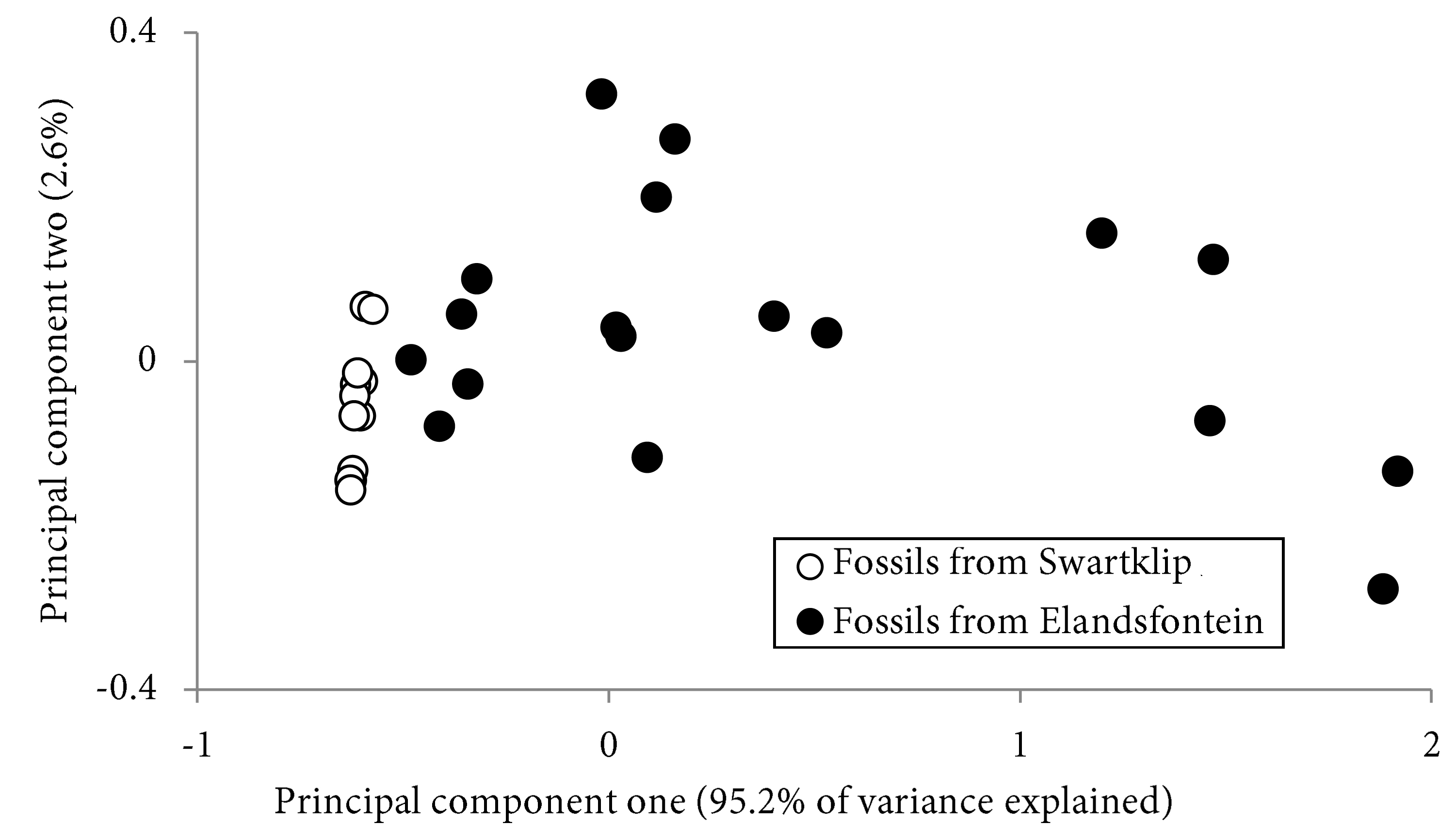
Principal component one and two score values. Each score value represents a fossil antelope bone from South Africa. Modified from Thomas and Chinsamy 2011.

We found that our Fe and Sr peaks were positively loaded. In our scores plot, this means that samples with positive PC1 scores should be rich with Fe and Sr. Likewise, our Ca peaks were negatively weighted, and so our samples with negative PC1 scores probably contain an extra calcite mineral. If we take a look at our PC1 scores we find that the positively weighted samples are all from Elandsfontein Main, and all of the Swartklip 1 have negative score values.

So we have found a chemical difference between the bones of these two sites. Elandsfontein bones have been infiltrated with iron and strontium rich minerals, which actually turn out to be clays and sands deposited by groundwater. The Swartklip bones contain abundant calcite. What does that mean for the burial history of these two sites?

The fossil bones at Elandsfontein Main and Swartklip 1 both accumulated in dune environments during the Pleistocene. The Elandsfontein Main site remained inland, and the slightly acidic groundwater that percolated through the fossils partially dissolved the bones and filled them with sediment. In contrast, sea level change periodically brought the coastline close to the Swartklip 1 site, where it is now, actually. The marine influence introduced calcium carbonate into the environment, which buffered the acidic groundwater and laced it with dissolved carbonates. These carbonates precipitated onto the Swartklip 1 fossils.

So, at Elandsfontein Main we have fossils that have been subjected to acidic groundwater for tens of thousands of years, and at Swartklip 1, we have fossils that have been periodically buffered by soil carbonates. If I was to pick one site to start looking for intact and well preserved bone, even down to isotope-level, I would start with the fossils Swartklip 1.

So yeah, this is the type of information we get from spectroscopy and principal components analysis. Pretty cool eh.

Thomas D B, Chinsamy A, 2011. Chemometric analysis of EDXRF measurements from fossil bone. X-ray Spectrometry 40: 441-445

Still to come: R code for pretreating spectra, performing a PCA analysis, and producing informative graphs…

#PCA is your friend

X-ray diffraction spectrum of calcite, the mineral that makes up most fossil shells. Data from The RRUFF™ Project

Most of the chemical tools we use to study fossils produce a data spectrum, which is just a set of measurements made over a series of observations. For example, think of the output from an x-ray diffraction analysis – the pattern of peak counts for each two-theta value is a spectrum. Other instruments that produce spectra include x-ray fluorescence, isotope ratio mass spectrometry, Fourier transform infrared spectroscopy and so on. We have become adept at reducing these data spectra to a single or few values of interest – calcite has an intense two-theta value at 29.4 under irradiation from a copper source – and we tend to throw away the rest of the spectrum. While there are study questions that can be addressed with point values (“Is there calcite in my fossil clam shell?”), there are other questions that could be better answered while working with the whole spectrum. Is there more than just calcite in my fossil shell? Does the calcite have an unusual chemistry? Is my fossil shell different to your fossil shell? These are questions that we can address by looking at variation between spectra, which we can do with principal component analysis.

I am going to switch study systems and talk about fossil bones and x-ray fluorescence. I will work this up as a practical  tutorial of sorts, and talk about some data from South African fossils that I collected a couple of years ago. There are a couple of advantages in working with these data – one, this is a real world scenario with a tangible result – two, the spectral data are available online so you can perform your own principal component analyses on fossil data.

Principal component analysis (PCA) on spectra from fossil bones.

Premise: Stable isotopes in fossils are an incredibly rich source of information about ancient animals. Isotopes in fossil teeth and bones can tell us what an animal ate and how frequently it visited a source of water. Unfortunately, teeth and bones can become altered when they are buried, and the important biological information in the isotopic compositions can be lost. It would be nice to know ahead of time whether or not a fossil bone is altered, and one approach to assessing alteration is to study the burial history of the fossil bone or tooth. In this scenario we are going to examine the burial history of a fossil by studying the elemental composition of the fossil surface – changes in the environment over time will have changed the chemistry of the fossil. We will study fossils from two different Pleistocene locations in the Western Cape of South Africa, and the end goal is to decide which location has the best-preserved fossils.

Samples: Fossil teeth and bones from two localities were analysed. These bones were the horn cores of Pleistocene antelope – springbok (Antidorcas marsupialis), eland (Taurotragus oryx) and a relative of sable (Hippotragus sp.).

Data collection: Fossil teeth and horn cores from each site were analysed with a portable x-ray fluorescence instrument. We will use the energy spectra that the instrument produced, rather than the elemental ratios.

Swartklip fossil location, outside of Cape Town South Africa

Elandsfontein fossil location, outside of Cape Town South Africa

 

Results and Discussion: A principal component analysis (PCA) identifies the sources of variation in a dataset, which it sees as individual ‘components’. The largest source of variation is principal component one, the second largest source of variation is principal component two, and so on. By separating out sources of variation, PCA provides us with two very important sets of data about the samples we have analysed.

The first set of data are the ‘score values’ (or eigenvalues). The spectrum from each sample is reduced to a single ‘score’ value for each principal component. Samples will have similar score values when they have similar amounts of a particular variable . So, we can look at a distribution of score values and see which samples are more similar to which other samples by how closely positioned they are. Lets take this image here:

Principal component score values, from XRF analyses of fossil bones and teeth.

These are the score values from principal component one and principal component two, for our fossil XRF data. The first thing to notice is that all of the Swartklip samples have similar PC1 values. That is, the fossils from the two sites can be separated by the variation that is being pulled out by principal component one. The fossils from both sites have a range of PC2 values, so there is variation at both sites in whatever this component is. So, what is the source of variation along principal component one that is separating these fossil sites?

More soon, including the R code for pre-treating spectral data, performing PCA, and presenting PCA results…